Analyzing and forecasting with time series data using ARIMA models in Python

The ARIMA algorithm (ARIMA stands for Autoregressive Integrated Moving Average) is used for time series analysis and for forecasting possible future values of a time series. Autoregressive modeling and Moving Average modeling are two different approaches to forecasting time series data. ARIMA integrates these two approaches, hence the name. ARIMA is one of the most widely used approaches to time series forecasting and it can be used in different ways depending on the type of time series data that you're working with.

Forecasting is a branch of machine learning using the past behavior of a time series to predict the one or more future values of that time series. Imagine that you're buying ice cream to stock a small shop. If you know that sales of ice cream have been rising steadily as the weather warms, you should probably predict that next week's order should be a little bigger than this week's order. How much bigger should depend on the amount that this week's sales differ from last week's sales. We can't forecast the future without a past to which to compare it, so past time series data is very important for ARIMA and for all forecasting and time series analysis methods.

In this tutorial we'll use what's known as the Box-Jenkins method of forecasting. The approach starts with the assumption that the process that generated the time series can be approximated using an ARMA model if it is stationary. This method consists of four steps:

1. Identification: Assess whether the time series is stationary, and if not, how many differences are required to make it stationary. Then, generate differenced data for use in diagnostic plots. Identify the parameters of an ARIMA model for the data from auto-correlation and partial auto-correlation.

2. Estimation: Use the data to train the parameters (that is, the coefficients) of the model.

3. Diagnostic Checking: Evaluate the fitted model in the context of the available data and check for areas where the model can be improved. In particular, this involves checking for overfitting and calculating the residual errors.

4. Forecasting: Now that you have a model, you can begin forecasting values with your model.

In this tutorial you'll learn about how ARIMA models can help you analyze and create forecasts from time series data. You'll learn how to create and assess ARIMA models using several different Python libraries in a Jupyter notebook on the IBM watsonx.ai platform with a data set from the US Federal Reserve.

Prerequisites

You need an IBM Cloud account to create a watsonx.ai project.

Steps

Step 1. Set up your environment

While you can choose from several tools, this tutorial walks you through how to set up an IBM account to use a Jupyter Notebook. Jupyter Notebooks are widely used within data science to combine code, text, images, and data visualizations to formulate a well-formed analysis.

1. Log in to watsonx.ai using your IBM Cloud account.

2. Create a watsonx.ai project.

3. Create a Jupyter Notebook.

This step will open a Notebook environment where you can load your data set and copy the code from this tutorial to perform the time series analysis and ARIMA modeling.

Step 2. Install and import libraries

We’ll use several libraries for creating our ARIMA models. First, the sktime library, a Python library for time series analysis and learning tasks such as classification, regression, clustering, annotation, and forecasting. Second, seaborn which is a library for data visualization and the creation of charts. You'll use matplotlib to interact with additional plots. The pandas library is the canonical library for working with loaded data in Python. The statsmodels library will be used to create our ARIMA models and provides utilities for visualization as well. Finally the pmdarima library provides an implementation of automatic ARIMA that we can use to discover optimal settings for the ARIMA model.

%pip install sktime seaborn matplotlib pandas statsmodels pmdarima;

Now that we've installed all of the libraries, we can import them into our environment:

import sktime
from matplotlib import pyplot
import matplotlib as plt
import seaborn
import datetime
import pandas as pd
import statsmodels

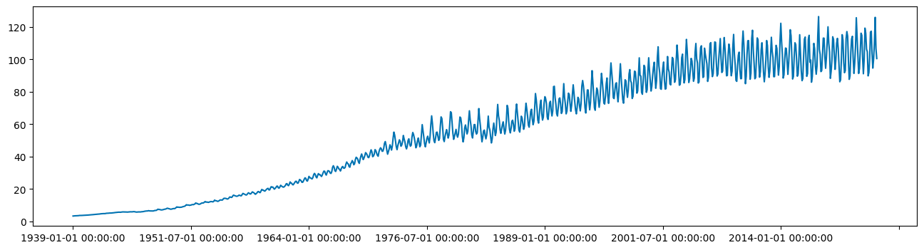
The data we'll use in this example is from the US Federal Reserve and is available here. You can either download the data directly to a local machine and then upload it to your watsonx environment or run the command below. We create the Pandas dataframe and then create a datetime index for the dataframe so that we can more easily work with it in sktime.

url = "https://fred.stlouisfed.org/graph/fredgraph.csv?bgcolor=%23e1e9f0&chart_type=line&drp=0&fo=open%20sans&graph_bgcolor=%23ffffff&height=450&mode=fred&recession_bars=on&txtcolor=%23444444&ts=12&tts=12&width=1318&nt=0&thu=0&trc=0&show_legend=yes&show_axis_titles=yes&show_tooltip=yes&id=IPG2211A2N&scale=left&cosd=1939-01-01&coed=2024-03-01&line_color=%234572a7&link_values=false&line_style=solid&mark_type=none&mw=3&lw=2&ost=-99999&oet=99999&mma=0&fml=a&fq=Monthly&fam=avg&fgst=lin&fgsnd=2020-02-01&line_index=1&transformation=lin&vintage_date=2024-05-07&revision_date=2024-05-07&nd=1939-01-01"

# change for your uploaded URL
df = pd.read_csv(url, parse_dates=['DATE'])
df.columns = ['date', 'production']
df['date'] = pd.to_datetime(df['date'])
df = df.set_index(df['date']).drop('date', axis=1)
df.head()

Here, you can see the first 5 rows of the dataframe.

date            production
1939-01-01    3.3336
1939-02-01    3.3591
1939-03-01    3.4354
1939-04-01    3.4609
1939-05-01    3.4609

The statsmodels library requires that our dataframe have an explicit temporality, so resample the data with 'MS' to ensure that the dataframe knows that the data is using a Month Start interval.

df = df.resample("MS").last()

Step 3. Load the data and perform EDA

Before we start estimating what kind of ARIMA model, do some quick exploratory data analysis.

First, we can look at the statistics of our data set.

df.describe().T

There's quite a wide standard deviation, which may indicate some non-stationarity in the time series. Plotting the time series can also help show trend and seasonality.

from sktime.utils.plotting import plot_series
plot_series(df, markers=' ')

Step 4. Check stationarity and variance

Now, we need to establish whether our time series model is stationary or not. ARIMA models can handle cases where the non-stationarity is due to a unit-root but may not work well at all when non-stationarity is of another form.

There are three basic criteria for a series to be classified as stationary series. First, the mean of the series should not be a function of time, this means that the mean should be roughly constant though some variance can be modeled. Second, the variance of the series should not be a function of time. This property is known as homoscedasticity. Third, the covariance of the terms, for example the k^th term and the (k + n)^th term, should not be a function of time.

Essentially a stationary time series is a flat looking series, without trend, constant variance over time, a constant autocorrelation structure over time, and no periodic fluctuations. It should resemble white noise as closely as possible. It’s fairly evident that our time series is non-stationary so our model will likely need to reflect that.

We can confirm that our time series is non-stationary by using two tests: the Augmented Dickey-Fuller (ADF) test and the Kwiatkowski-Phillips-Schmidt-Shin (KPSS) test. First, the ADF test. This is a type of statistical test called a unit root test. The ADF test is conducted with the following assumptions:

• The null hypothesis for the test is that the series is non-stationary, or series has a unit root.
• The alternative hypothesis for the test is that the series is stationary, or series has no unit root.

If the null hypothesis cannot be rejected, then this test may provide evidence that the series is non-stationary. This means that when you run the ADF test, if the test statistic is less than the critical value and p-value is less than 0.05, then we reject the null hypothesis, which means the time series is stationary.

from statsmodels.tsa.stattools import adfuller

adf_result = adfuller(df)
print(adf_result[1])

0.8251271628322037

We can see that the data is not currently stationary because the ADF test value is above 0.05. Running the KPSS test can help confirm this.

from statsmodels.tsa.stattools import kpss

kpss_result = kpss(df)
print(kpss_result[1])

0.01

Here the KPSS test also indicates that our time series is not stationary becauase the KPSS test result is below 0.05.

Having two tests which may or may not agree can be confusing. If KPSS and ADF agree that the series is stationary then we can consider it stationary and there’s no need to to use a difference term in the ARIMA model.

If the ADF test finds a unit root but KPSS finds that the series is stationary around a deterministic trend then the series is trend-stationary, and it needs to be detrended. You can either difference the time series by using the diff method or a Box-Cox transformation may remove the trend.

If the ADF does not find a unit root but KPSS claims that it is non-stationary then the series is difference stationary. We'll need to difference the data before passing data to our autoregressive model.

If KPSS and ADF agree that the series is non-stationary then we can consider it non-stationary. We'll need to difference the data before passing data to our autoregressive model.

We'll use the decompose method to determine what may need to be removed from the time series in order to fix it.

from statsmodels.tsa.seasonal import seasonal_decompose

result = seasonal_decompose(df, model='additive')
result.plot()
pyplot.show()

Since this is a little difficult to see we can run the decompose function on a subset of the data, in this case only seeing the first 48 months of the data set.

result = seasonal_decompose(df[:48], model='additive')
result.plot()
pyplot.show()

The naive decomposition method is a simple one and there are more advanced decompositions available like Seasonal and Trend decomposition using Loess or STL decomposition. We don't want to make too many strong inferences from the results of this output. It does in this case though show us that there is a strong trend and seasonality present.

We can see that our time series contains trend and seasonal components but also that the variance of the time series is increasing over time. ARIMA models handle seasonality and non-stationarity well but they don't handle changes in variance or heteroskedasticity especially well.

When we encounter heteroskedasticity in a time series it's common to take a log transformation to manage it. One tool for doing this is the Box-Cox transformation. The boxcox method takes a lambda parameter which is defined as follows:

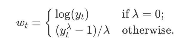
We can apply a Box-Cox transformation to the data with the boxcox method.

from scipy.stats import boxcox
from scipy.special import inv_boxcox

df['production'],fitted_lambda= boxcox(df['production'],lmbda=None)
plot_series(df['production'], markers=' ')

df.head()

This will return the first five rows of the data set.

production
1939-01-01    1.799502
1939-02-01    1.815773
1939-03-01    1.864188
1939-04-01    1.880279
1939-05-01    1.880279

Now the trend is still present, but the variance has decreased enough that we can investigate how ARIMA models will fit our data.

Step 5. Plot auto-correlations

First, create a test train split that can be used both train our model and then test the efficacy of that model. We'll hold out the last 24 values of the data set as a testing set.

from sktime.split import temporal_train_test_split
train, test = temporal_train_test_split(df, test_size=36)

Next, we need to check to see where our de-trended time series data contains autocorrelations. We can see the degree to which a time series is correlated with its past values by calculating the auto-correlation. Calculating the autocorrelation can answer questions about whether the data exhibit randomness and how related one observation is to an immediately adjacent observation. This can give us a sense of what sort of model might best represent the data. The autocorrelations are often plotted to see the correlation between the points up to and including the lag unit. There are two approaches to autocorrelations: the autocorrelation function (ACF) and the partial autocorrelation function (PACF).

In ACF, the correlation coefficient is in the x-axis whereas the number of lags (referred to as the lag order) is shown in the y-axis. In Python, we can use the autocorrelation_plot function to create an auto-correlation plot.

from pandas.plotting import autocorrelation_plot
autocorrelation_plot(train[-24:])

Across 24 time units, the detrended series still shows a positive but decreasing correlation at lags 6, 12, and 18 and a negative and decreasing correlation at lags 3, 9, and 15. This would indicate that our time series still has a seasonality component to it. The only one that is outside of the critical range of 0.5 to -0.5 though is at 3, so that might indicate a value for the autoregressive component of our ARIMA model.

It is also a good idea to check the Partial Autocorrelation Function (PACF) as well. A partial correlation is a conditional correlation. As an example, think of a time series where the time series contains values for Y at X_t, X_t+1, and X_t+2. The partial correlation between Y and X_t+2 is the correlation between the variables determined taking into account how both Y and X_t+2 are related to X_t and X_t+1.

The PACF is helpful in determining the order of the AR part of the ARIMA model. It is also useful to determine or validate how many seasonal lags to include in the forecasting equation of a moving average based forecast model for a seasonal time series. This is called the seasonal moving average (SMA) order of the process.

from statsmodels.graphics.tsaplots import plot_pacf

plot_pacf(train[-48:])
pyplot.show()

Again, the value that is outside of the critical range of 0.5 to -0.5 though is at 3 so this indicates a value for the autoregressive component of our ARIMA model.

A rough rubric for when to use Autoregressive terms in the model is when:

• ACF plots show autocorrelation decaying towards zero
• PACF plot cuts off quickly towards zero
• ACF of a stationary series shows positive at lag 1

A rough rubric for when to use moving average terms in the model is when:

• The ACF is negatively autocorrelated at lag 1
• ACF that drops sharply after a few lags
• PACF decreases gradually rather than suddenly

We can see from our two plots that our ACF plot shows a positive value at lag 1 and that the PACF cuts off somewhat quickly. This might indicate that we should use an AR term in our model.

Step 6. Train the ARIMA model

Now that we have a sense of what kinds of ARIMA model might represent our data well, we can begin training a model.

First, we can call the arima function without a seasonal component, which has the following parameters:

ARIMA(dataset, order)

The order is a tuple with 3 values:

• p: the order of the autoregressive term
• d: degree of differencing
• q: the number of moving average terms

Since we saw characteristics in the ACF and PACF plots that might indicate an AR model, we'll create a first-order autoregressive model. We use the checkresiduals function to generate graphs of the residuals, the ACF, and the distribution of the residuals. We'll use an autoregressive term and a first difference term because our data exhibits non-stationarity.

from statsmodels.tsa.arima.model import ARIMA

model = ARIMA(train, order=(3,1,0))
model_fit = model.fit()

Now let's look at the summary of the generated model.

print(model_fit.summary())

This will output:

SARIMAX Results
    ==============================================================================
    Dep. Variable:             production   No. Observations:                  987
    Model:                 ARIMA(3, 1, 0)   Log Likelihood                -897.873
    Date:                Thu, 09 May 2024   AIC                           1803.745
    Time:                        08:05:04   BIC                           1823.320
    Sample:                    01-01-1939   HQIC                          1811.190
                             - 03-01-2021
    Covariance Type:                  opg
    ==============================================================================
                     coef    std err          z      P>|z|      [0.025      0.975]
    ------------------------------------------------------------------------------
    ar.L1          0.2336      0.018     13.347      0.000       0.199       0.268
    ar.L2         -0.2893      0.015    -19.328      0.000      -0.319      -0.260
    ar.L3         -0.5837      0.016    -36.730      0.000      -0.615      -0.553
    sigma2         0.3609      0.010     35.557      0.000       0.341       0.381
    ===================================================================================
    Ljung-Box (L1) (Q):                  46.72   Jarque-Bera (JB):               689.49
    Prob(Q):                              0.00   Prob(JB):                         0.00
    Heteroskedasticity (H):              53.41   Skew:                            -0.22
    Prob(H) (two-sided):                  0.00   Kurtosis:                         7.07
    ===================================================================================

There is a lot to look at here. We can see the coefficients for the model specification and some of the calculated statistics for it:

• sigma²: this represents the variance of the residual values, lower is better
• log likelihood: this is maximum likelihood estimation for the ARIMA model, higher is better
• aic: a measure of the goodness of fit and the parsimony of the model, lower is better

Let’s plot the residuals to ensure there are no patterns in them. We're hoping for a constant mean and variance.

# density plot of residuals
residuals = pd.DataFrame(model_fit.resid)
fig, ax = pyplot.subplots(1,2, figsize=(14, 6))
residuals.plot(title="Residuals", ax=ax[0])
residuals.plot(kind='kde', title='Density', ax=ax[1])
pyplot.show()

We can see that as the variance increases, so do the residuals but this may simply be a feature of our data. It's time to see how the predictive power of the fitted model matches the test data. The test data can be added one time point at a time to the train data to allow the model to include the new data point in the training.

history = train
predictions = list()
# walk-forward validation
for t in range(len(test),0,-1):
    model = ARIMA(df[:-t], order=(3,1,0));
    model_fit = model.fit();
    output = model_fit.forecast();
    yhat = output.iloc[0]
    predictions.append(yhat)

The output predictions are stored in a list called predictions so that the predictions can be graphed alongside the actual test values.

test.loc[:,'predictions'] = predictions.copy()

pyplot.plot(test['predictions'], color='red', label='prediction')
pyplot.plot(test['production'], color='blue', label='actual')
pyplot.legend(loc="upper left")
pyplot.xticks(rotation=45)
pyplot.show()

Let's check the root mean squared error.

from sklearn.metrics import mean_squared_error
from math import sqrt

# evaluate forecasts
rmse = sqrt(mean_squared_error(test['predictions'], test['production']))
print('Test RMSE: %.3f' % rmse)

This will output:

Test RMSE: 1.171

We can see a root mean squared error of 1.171. One feature of the original data set that our model isn't addressing is the seasonality. Another technique for creating ARIMA models is to use an Auto ARIMA implementation that creates a model for us.

Seasonal autoregressive integrated moving average, SARIMA or Seasonal ARIMA, is an extension of ARIMA that supports time series data with a seasonal component. To do this, it adds three new hyperparameters to specify the autoregression, differencing and moving average for the seasonal component of the series, as well as an additional parameter for the period of the seasonality. A SARIMA model is typically expressed SARIMA((p,d,q),(P,D,Q)), where the lower case letters indicate the non-seasonal component of the time series and the upper case letters indicate the seasonal component

The pmdarima library provides access to an auto-ARIMA process which seeks to identify the most optimal parameters for an ARIMA model, settling on a single fitted ARIMA model. In order to find the best model, auto-ARIMA optimizes for a given information_criterion, one of Akaike Information Criterion, Corrected Akaike Information Criterion, Bayesian Information Criterion, Hannan-Quinn Information Criterion, or “out of bag” (for validation scoring), respectively, and returns the ARIMA which minimizes the value.

To determine the order of differencing, d, and then fitting models within ranges of defined start_p, max_p, start_q, max_q ranges. If the seasonal optional is enabled, auto-ARIMA also seeks to identify the optimal P and Q hyperparameters after conducting the Canova-Hansen to determine the optimal order of seasonal differencing, D.

import pmdarima as pm

auto_model = pm.auto_arima(train, start_p=1, start_q=1,
                      test='adf', # use adftest to find optimal 'd'
                      m=12, # frequency of series
                      d=None, # let model determine 'd'
                      seasonal=True, # Use Seasonality
                      information_criterion='aicc',
                      error_action='ignore',
                      suppress_warnings=True,
                      stepwise=True)

Now we can see the summary for the discovered optimal model.

print(auto_model.summary())

This will output the summary of the model parameters and statistics:

SARIMAX Results
    ===============================================================================================
    Dep. Variable:                                       y   No. Observations:                  987
    Model:             SARIMAX(2, 1, 1)x(2, 0, [1, 2], 12)   Log Likelihood                -337.822
    Date:                                 Fri, 10 May 2024   AIC                            691.644
    Time:                                         07:52:31   BIC                            730.793
    Sample:                                     01-01-1939   HQIC                           706.534
                                              - 03-01-2021
    Covariance Type:                                   opg
    ==============================================================================
                     coef    std err          z      P>|z|      [0.025      0.975]
    ------------------------------------------------------------------------------
    ar.L1          0.5714      0.025     22.922      0.000       0.523       0.620
    ar.L2         -0.0517      0.024     -2.119      0.034      -0.099      -0.004
    ma.L1         -0.9270      0.014    -66.600      0.000      -0.954      -0.900
    ar.S.L12       0.5686      0.158      3.599      0.000       0.259       0.878
    ar.S.L24       0.4225      0.156      2.710      0.007       0.117       0.728
    ma.S.L12      -0.1818      0.156     -1.164      0.244      -0.488       0.124
    ma.S.L24      -0.4028      0.096     -4.203      0.000      -0.591      -0.215
    sigma2         0.1126      0.004     32.170      0.000       0.106       0.119
    ===================================================================================
    Ljung-Box (L1) (Q):                   0.00   Jarque-Bera (JB):               357.52
    Prob(Q):                              0.99   Prob(JB):                         0.00
    Heteroskedasticity (H):              43.17   Skew:                            -0.00
    Prob(H) (two-sided):                  0.00   Kurtosis:                         5.95
    ===================================================================================

We can see that the model is SARIMAX(2, 1, 1)x(2, 0, [1, 2], 12), which means that the non-seasonal components are 2, 1, 1, and the seasonal components are 2, 0, [1,2].

The AIC of the generated SARIMA model is less than half of the non-seasonal model we created previously. This could indicate that the seasonal component is an important feature for our modeling. The plot_diagnostics method can help us see residuals of the model, the histogram of errors, a Q-Q normality plot, and a correlation plot of the errors called a correlogram.

auto_model.plot_diagnostics(figsize=(14, 6))
pyplot.show()

Now we'll create a prediction of the data set but without retraining for each new data point in the test set. We'll simply ask the auto_model to output 36 predictions.

history = train
auto_predictions = auto_model.predict(len(test))

Again, we'll graph the predictions and the actual test values.

test.loc[:, 'auto_predictions'] = auto_predictions.copy()

pyplot.plot(test['auto_predictions'], color='red', label='prediction')
pyplot.plot(test['production'], color='blue', label='actual')
pyplot.legend(loc="upper left")
pyplot.show()

Checking the RMSE we can see an RMSE of 0.587, less than half of the non-seasonal model.

# evaluate forecasts
rmse = sqrt(mean_squared_error(test['auto_predictions'], test['production']))
print('Test RMSE: %.3f' % rmse)

This will output:

Test RMSE: 0.587

We can see that the RMSE for our Seasonal ARIMA model is much smaller than for the non-Seasonal ARIMA model.

Summary and next steps

In this tutorial, we've learned about the ARIMA algorithm and how we can use it to forecast time series data. We learned to test for stationarity and homoskedasticity in a time series and how to transform a time series in order to correct the variance in the time series dataset. We fit multiple ARIMA models and compared them using the AIC metric and the RMSE of the forecasts. You also learned about the Auto-ARIMA method to generate a model by automatically comparing values of d to minimize the stationarity and values of p and d to minimize AIC.

Try watsonx for free

Build an AI strategy for your business on one collaborative AI and data platform called IBM watsonx, which brings together new generative AI capabilities, powered by foundation models, and traditional machine learning into a powerful platform spanning the AI lifecycle. With watsonx.ai, you can train, validate, tune, and deploy models with ease and build AI applications in a fraction of the time with a fraction of the data.

Try watsonx.ai, the next-generation studio for AI builders.

Next steps

Explore more articles and tutorials about watsonx on IBM Developer.